Triple-Barrier Method & Meta-Labeling: Machine Learning for Crypto Quants

📚 Serial: Quantitative Crypto Trading Mastery 2026 (Part 2/6)

Market Microstructure & Dollar Bars — The Foundation

👉 Triple-Barrier Method & Meta-Labeling — Machine Learning for Quants (you are here)

Kelly Criterion & Perpetual Funding Rate — Mathematical Sizing & Risk

Mastering CoinXSight Quant Terminal — The 4-Step Decision Pipeline

Tracking Whale Flow with Dollar Bars — VWAP & Tick Count Analysis

Liquidation Squeeze & Microstructure Playbook — Live Derivatives Trading

---

Why Standard Machine Learning Fails in Financial Markets

When data scientists first enter cryptocurrency algorithmic trading, they almost universally apply textbook machine learning workflows:

1. Sample price data into fixed time bars (e.g., 5-minute candles).
2. Assign a binary label based on future return after a fixed horizon:
3. Train an XGBoost model or neural network using standard k-fold cross-validation.
4. Observe an impressive backtested Sharpe ratio of 3.8 — followed by catastrophic capital drawdown in live production.

This failure mode is not caused by weak algorithms; it is caused by structural flaws in data preparation, labeling, and validation. Financial time series violate the fundamental assumption of machine learning: Independent and Identically Distributed (I.I.D.) observations.

In this guide, we explore the institutional machine learning architecture pioneered by Marcos López de Prado in Advances in Financial Machine Learning (Wiley, 2018): the Triple-Barrier Method, Meta-Labeling, and Combinatorial Purged Cross-Validation (CPCV).

---

The Flaw of Fixed-Horizon Labeling

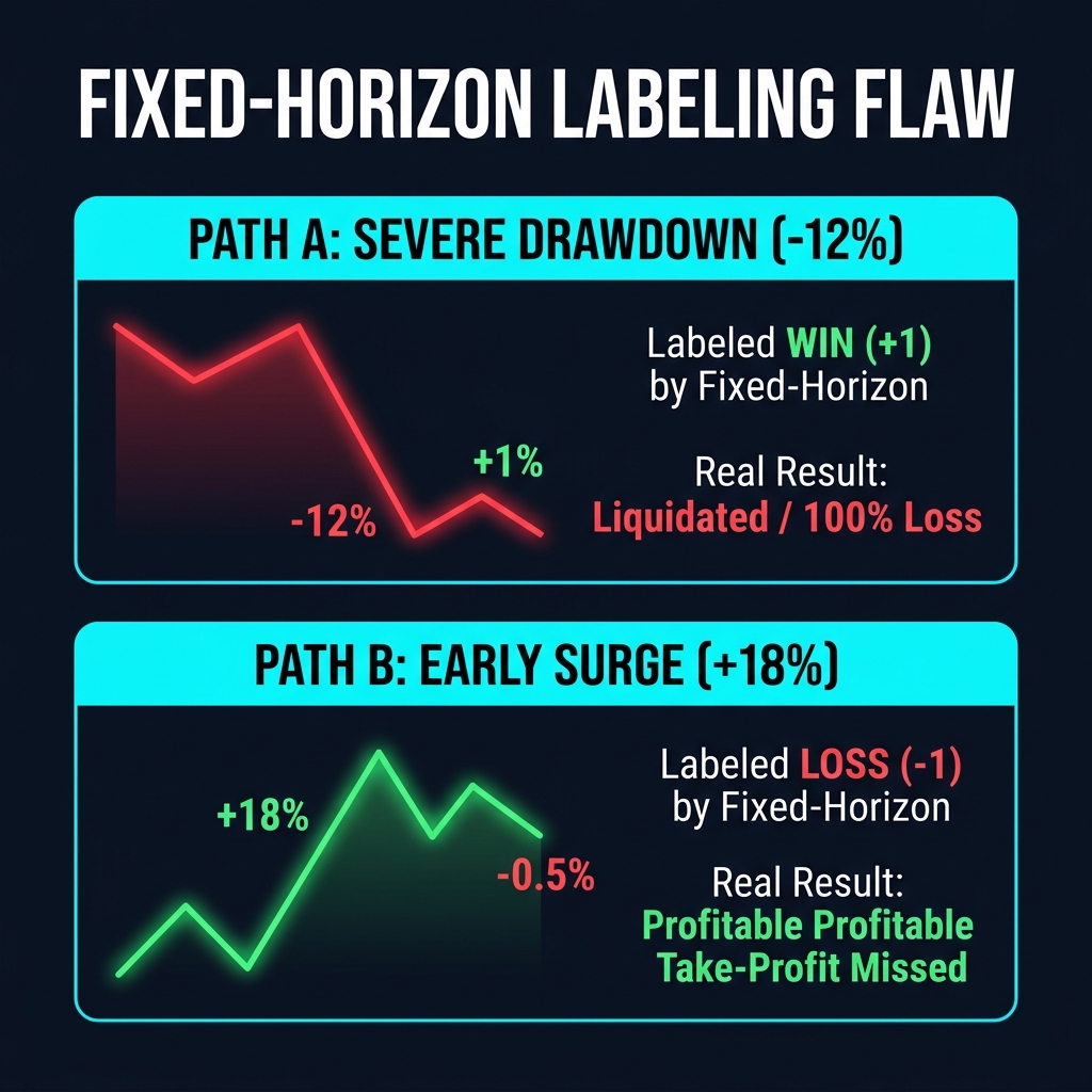
Consider a standard fixed-horizon rule where a model attempts to predict price movement 20 bars into the future (t + 20).

In live trading, real market participants do not hold positions blindly until a stopwatch rings. They use Take-Profit (TP) and Stop-Loss (SL) orders.

• Path A would have bankrupted the trader long before t+20.
• Path B captured substantial alpha that an arbitrary time-based evaluation discarded.

Fixed-horizon labeling completely ignores the path of prices, introducing severe mislabeling bias that cripples model learning.

---

The Triple-Barrier Method: Path-Dependent Labeling

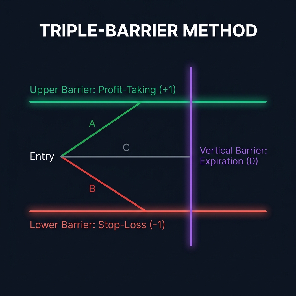
To reflect real-world market dynamics, the Triple-Barrier Method bounds every trade by three dynamic frontiers:

The Three Barriers

1. Upper Horizontal Barrier (Profit Target π+): The profit-taking target. Dynamic threshold set as a multiple of rolling volatility: Profit Target = Entry × (1 + k_pt × Rolling Volatility σ)
2. Lower Horizontal Barrier (Stop Loss π-): The stop-loss threshold, similarly anchored to asset volatility: Stop Loss = Entry × (1 - k_sl × Rolling Volatility σ)
3. Vertical Barrier (Expiration t1): The maximum holding period (e.g., 20 dollar bars). If neither the upper nor lower barrier is touched before $t_1$, the position is closed at market price.

Volatility-Anchored Dynamic Thresholds

In crypto, daily volatility swings from 1.5% during consolidation to 8.5% during liquidity cascades. A static 2% take-profit target is unachievable during low-volatility regimes and prematurely closed during momentum breakouts.

By scaling barriers with an exponential moving standard deviation of returns (rolling volatility σ), the Triple-Barrier Method maintains constant statistical difficulty across varying market regimes:

# Conceptual implementation of dynamic barrier setting
def compute_daily_volatility(close_prices, span=100):
    returns = close_prices.pct_change()
    return returns.ewm(span=span).std()

---

Meta-Labeling: Decoupling Direction from Sizing

Traditional trading models force a single machine learning model to solve two completely distinct tasks simultaneously:

1. Will the price go up or down? (Directional Classification)
2. Should I take this trade, and how much capital should I allocate? (Bet Sizing & Confidence)

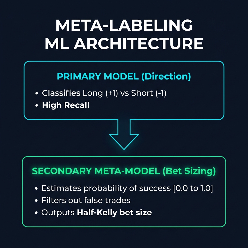
De Prado resolved this via Meta-Labeling — an institutional two-stage architecture:

+──────────────────────────────────────────────────────────────────────────+
|  PRIMARY MODEL (Heuristic / Rule-Based / High Recall)                    |
|  - Microstructure signals: OBI skew, VWAP cross, Dollar-bar imbalance   |
|  - Output: Directional Bet (Long = +1, Short = -1)                       |
+────────────────────────────────────┬─────────────────────────────────────+
                                     │
                                     ▼
+──────────────────────────────────────────────────────────────────────────+
|  SECONDARY MODEL (Machine Learning / High Precision Meta-Model)           |
|  - Features: Volatility, Market Regime, Funding Skew, Order Flow Delta    |
|  - Target: Binary outcome (1 = Primary Model hit TP; 0 = Hit SL/Timeout) |
|  - Output: Probability p ∈ [0.0, 1.0]                                    |
+────────────────────────────────────┬─────────────────────────────────────+
                                     │
                                     ▼
+──────────────────────────────────────────────────────────────────────────+
|  BET SIZING ENGINE (Sigmoid Mapping & Fractional Kelly)                  |
|  - Size = f(Probability p, Volatility σ)                                 |
+──────────────────────────────────────────────────────────────────────────+

Advantages of Meta-Labeling

• Overcoming Class Imbalance: Primary models can be tuned for high recall (casting a wide net for opportunities), while the secondary meta-model acts as a strict risk filter (maximizing precision).
• Direct Bet Sizing: The meta-model's output probability $p$ directly informs position sizing. A trade with p = 0.52 receives minimal allocation, whereas p = 0.88 commands high conviction capital.
• Preserving Interpretability: Traders retain clear rule-based logic for why an asset was selected, while letting non-linear ML govern risk exposure.

---

Preventing Leakage: Purging & Embargoing

Standard $k$-fold cross-validation randomly shuffles observations into train and test splits. In financial data with path-dependent labels, this creates catastrophic Information Leakage:

Training Sample (t = 10 to t = 30)  <────── OVERLAP ──────>  Testing Sample (t = 25)
                  Labels determined by future prices up to t=30!

Because an observation at $t = 10$ using the Triple-Barrier Method may not expire until $t = 30$, training a model on data that overlaps with the test set allows the model to "peek" into the future.

Purging

Purging eliminates any training observation whose labeling window overlaps with the test evaluation window:

[ Train Set ] ---[ PURGED GAP ]---> [ Test Set ]

Embargoing

Furthermore, because financial time series exhibit serial correlation (autocorrelation in volatility and order flow), observations immediately following the test set carry memory of the test environment. Embargoing removes a buffer (typically 1–2% of the dataset) immediately after the test split:

[ Train Set 1 ] ---> [ Test Set ] ---> [ EMBARGO ] ---> [ Train Set 2 ]

---

Combinatorial Purged Cross-Validation (CPCV)

Rather than evaluating a strategy on a single historical backtest path (which suffers from selection bias), quants employ Combinatorial Purged Cross-Validation (CPCV).

CPCV splits historical data into N chronological groups and generates all combinations of k testing groups. For $N = 6$ and $k = 2$, this generates 15 (6 choose 2) distinct backtested equity curves.

Split 1: [Test ][Test ][Train][Train][Train][Train]
Split 2: [Test ][Train][Test ][Train][Train][Train]
Split 3: [Test ][Train][Train][Test ][Train][Train]
...
Split 15:[Train][Train][Train][Train][Test ][Test ]

By analyzing the distribution of Sharpe ratios across all combinatorial paths, quants compute the Deflated Sharpe Ratio (DSR) — mathematically adjusting for data-snooping and trial count to verify true statistical edge.

---

Summary Architecture for Quantitative ML

1. Information Sampling: Convert raw trades into fixed $1,000,000 Dollar Bars.
2. Primary Signal: Generate directional hypothesis using order book microstructure or trend regimes.
3. Triple-Barrier Labeling: Set dynamic profit target (Profit Target π+) and stop loss (Stop Loss π-) anchored to rolling EWMA volatility.
4. Meta-Model Training: Train a classifier to predict whether the primary signal achieves its barrier, applying strict Purging and Embargoing.
5. Probability Sizing: Pass predicted probabilities into a fractional Kelly allocation engine.

💡 Next Steps: Once your model produces validated win probabilities, how do you size capital without risking catastrophic ruin?

Continue to Part 3: Kelly Criterion & Perpetual Funding Rate to master institutional bet sizing and crypto derivatives mechanics.