Neural Networks for Crypto Trading: From LSTMs to Transformers — What Actually Works

The Neural Network Hype vs. Reality

Every crypto AI project claims to use "advanced neural networks" and "deep learning." Most of them are running a basic LSTM from a 2019 tutorial, trained on 6 months of BTC price data, and calling it revolutionary.

Let's cut through the noise. Neural networks CAN work for crypto trading — but only when you understand which architecture matches which problem, how to avoid the catastrophic pitfalls, and what realistic performance looks like.

This guide is the honest technical breakdown. No hype. No "our AI predicted the crash" claims without evidence. Just what works, what doesn't, and why.

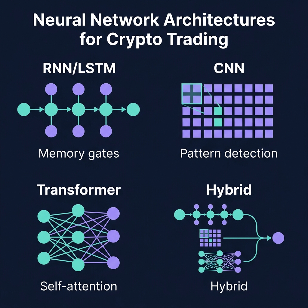
Neural Network Architectures for Crypto: The Complete Map

Architecture 1: Recurrent Neural Networks (RNNs) & LSTMs

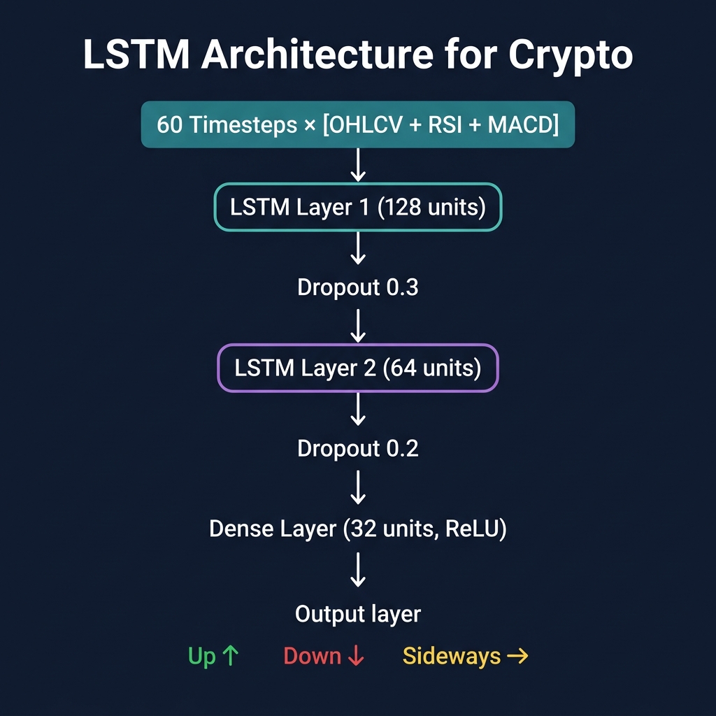
What they are: Networks designed for sequential data. Each step's output feeds into the next step's input, creating a "memory" of past data points.

LSTMs (Long Short-Term Memory) solve the "vanishing gradient" problem of basic RNNs by adding gates that control what information to remember, forget, and output.

Best for crypto:

• Short-term price direction prediction (1-24 hours)
• Volatility forecasting
• Detecting momentum regime changes

Typical LSTM architecture for crypto:

Input: [Open, High, Low, Close, Volume] × 60 timesteps (1-minute candles)
       + [RSI, MACD, Bollinger Width] × 60 timesteps
       
LSTM Layer 1: 128 units (captures short-term patterns)
Dropout: 0.3 (prevents overfitting)
LSTM Layer 2: 64 units (captures longer-term dependencies)
Dropout: 0.2
Dense Layer: 32 units + ReLU activation
Output: 3 units + Softmax (Up / Down / Sideways)

Realistic performance:

Metric	Typical Range	Good Performance
Direction accuracy (1h)	52-58%	> 55%
Direction accuracy (24h)	50-55%	> 53%
Sharpe ratio (backtest)	0.8-1.5	> 1.2
Sharpe ratio (live)	0.3-0.8	> 0.6

Why accuracy drops in live trading: Backtests don't include slippage, latency, and the fact that the model's predictions change the market if enough capital follows them. A 55% accurate model in backtest typically becomes 51-52% live — but that's still profitable with proper risk management.

Critical limitations:

• LSTMs struggle with sequences longer than ~200 timesteps — they "forget" earlier data
• Training on bull market data creates models that fail catastrophically in bear markets
• Extremely sensitive to input normalization — raw price data will not work

Architecture 2: Convolutional Neural Networks (CNNs)

What they are: Networks that apply sliding filters to detect patterns. Originally designed for images, but surprisingly effective for time-series data.

Why CNNs work for crypto:

Price charts ARE images — patterns like double bottoms, head-and-shoulders, and wedges are spatial patterns. CNNs can detect these patterns without being explicitly programmed to look for them.

Two approaches:

Approach A: 1D CNNs on raw data

Input: Price + indicator data as 1D time series
Conv1D Layer 1: 64 filters, kernel size 5 (captures 5-candle patterns)
Conv1D Layer 2: 128 filters, kernel size 3 (captures shorter patterns)
MaxPooling: Reduce dimensionality
Global Average Pooling → Dense → Output

Approach B: 2D CNNs on candlestick images

Input: Rendered candlestick chart as image (224×224×3)
Pre-trained ResNet50 backbone (transfer learning)
Custom head: Dense 256 → Dropout → Dense 3 (Up/Down/Sideways)

Realistic performance:

Metric	1D CNN	2D CNN (chart images)
Pattern detection accuracy	60-72%	65-78%
Direction prediction	52-56%	50-54%
Training speed	Fast (minutes)	Slow (hours)
Best use case	Feature extraction	Chart pattern recognition

Key insight: CNNs excel at pattern recognition but are weaker at sequence prediction. The best approach is to use CNNs as a feature extractor that feeds into a temporal model (LSTM or Transformer).

Architecture 3: Transformers

What they are: The architecture behind GPT, Claude, and every modern language model. Transformers use "self-attention" to weigh the importance of every timestep relative to every other timestep — no sequential processing needed.

Why Transformers are the future of crypto AI:

1. Unlimited lookback: Unlike LSTMs that forget after ~200 steps, Transformers can attend to thousands of timesteps simultaneously
2. Parallel processing: Train 10-50× faster than LSTMs because all timesteps are processed in parallel
3. Multi-modal inputs: Can combine price data, on-chain metrics, news sentiment, and social signals in a single model
4. Attention maps: Reveal WHICH historical patterns the model considers most important for its prediction — interpretable AI

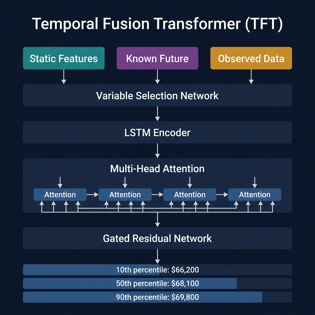
Temporal Fusion Transformer (TFT) — The Gold Standard:

The TFT is specifically designed for time-series forecasting and is the most effective Transformer architecture for crypto trading:

Input Features:
  Static: Asset type, exchange, sector
  Known future: Day of week, hour, funding schedule
  Observed: OHLCV, on-chain metrics, sentiment scores

Architecture:
  Variable Selection Network → selects which inputs matter
  LSTM Encoder → captures local temporal patterns  
  Multi-Head Attention → captures long-range dependencies
  Gated Residual Networks → controls information flow
  Quantile Output → predicts distribution, not point estimate

Why quantile output matters:

Instead of predicting "BTC will be $68,500 in 4 hours," TFT predicts:

• 10th percentile: $66,200 (worst case)
• 50th percentile: $68,100 (most likely)
• 90th percentile: $69,800 (best case)

This gives you a confidence range, not a single number. You can size your position based on the width of this range — narrow range = higher confidence = larger position.

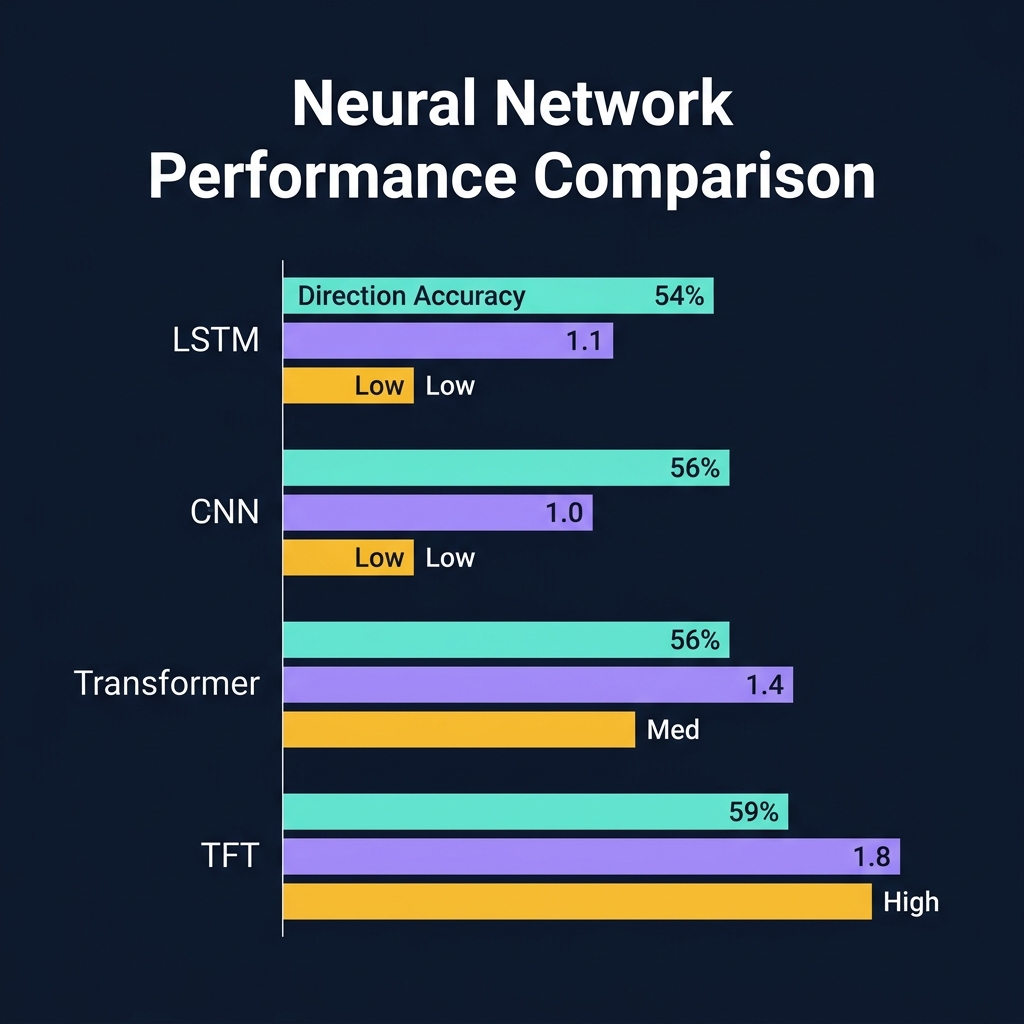
Realistic performance:

Metric	LSTM	Basic Transformer	TFT
MAE (4h prediction)	2.1%	1.8%	1.4%
Direction accuracy (4h)	54%	56%	59%
Sharpe (backtest)	1.1	1.4	1.8
Training time	2 hours	45 min	3 hours
Interpretability	Low	Medium	High

Architecture 4: Hybrid Models

The most effective production systems combine multiple architectures:

CNN-LSTM Hybrid:

CNN layers → extract spatial patterns from candlestick data
LSTM layers → model temporal dependencies across those patterns
Dense head → final prediction

This is like giving the model "eyes" (CNN) and "memory" (LSTM). The CNN sees chart patterns; the LSTM understands how those patterns evolve over time.

Transformer-CNN Hybrid:

CNN branch → processes candlestick images for chart patterns
Transformer branch → processes numerical time-series data
Fusion layer → combines both representations
Prediction head → output with confidence interval

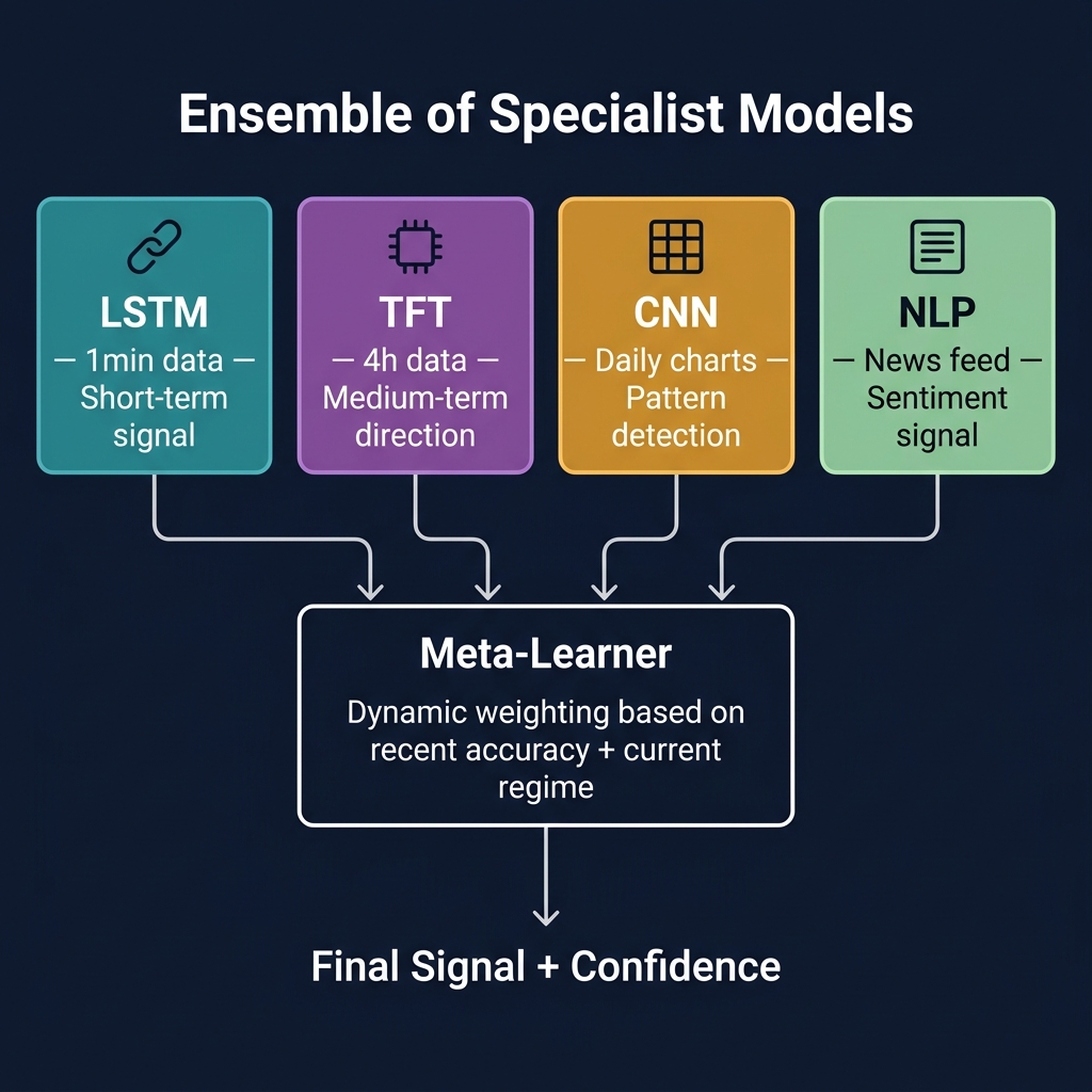
Ensemble of Specialists:

Model 1: LSTM on 1-minute data → ultra-short-term signal
Model 2: TFT on 4-hour data → medium-term direction
Model 3: CNN on daily charts → long-term pattern detection
Model 4: NLP model on news → sentiment signal

Meta-learner: Weighted combination based on each model's 
              recent accuracy and current market regime

CoinXSight's AI Analysis engine uses an ensemble approach — multiple specialist models whose outputs are combined by a meta-learner that weighs each model based on its recent track record.

The 7 Deadly Sins of Neural Network Trading

Understanding The 7 Deadly Sins of Neural Network Trading is a key part of crypto technical analysis. Most professional trading indicators on any crypto trading platform will help you apply these concepts in real time.

Sin 1: Training on Price Alone

Price data alone is insufficient. Neural networks need context to make useful predictions.

Minimum viable feature set:

Category	Features	Why
Price	OHLCV (5-minute, 1-hour, 4-hour, daily)	Core market data
Technical	RSI, MACD, ATR, Bollinger Bands, Volume Profile	Engineered patterns
On-chain	Active addresses, exchange flows, whale transactions	Fundamental demand
Sentiment	Social volume, fear/greed index, funding rates	Market psychology
Macro	DXY, S&P 500, US10Y yield, VIX	Cross-market correlation
Calendar	Hour of day, day of week, month, upcoming events	Temporal patterns

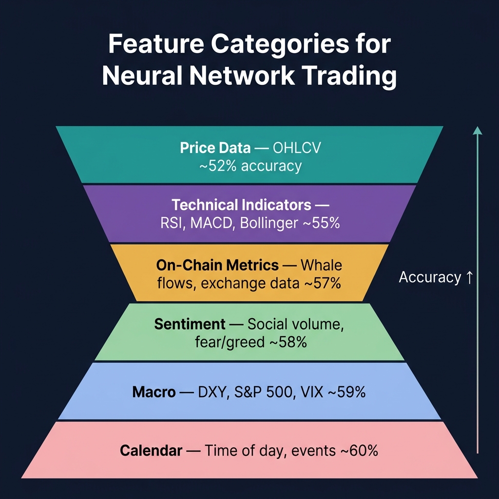
Models trained on OHLCV only achieve ~52% accuracy. Adding technical indicators pushes to ~55%. Adding on-chain + sentiment reaches ~58-60%. The marginal feature categories provide the edge.

Sin 2: Ignoring Non-Stationarity

Financial time series are non-stationary — their statistical properties change over time. A model trained on 2024 bull market data will fail in 2025's bear market because the patterns are fundamentally different.

Solutions:

1. Walk-forward training: Retrain the model every 1-4 weeks on a rolling window of data
2. Regime-aware training: Train separate models for different market regimes and use a classifier to select the right model
3. Stationary features: Instead of raw price, use returns (% change), log returns, or z-scores which are more stationary
4. Adaptive normalization: Normalize features using a rolling 30-day window instead of the entire training set

Sin 3: Overfitting to Backtest

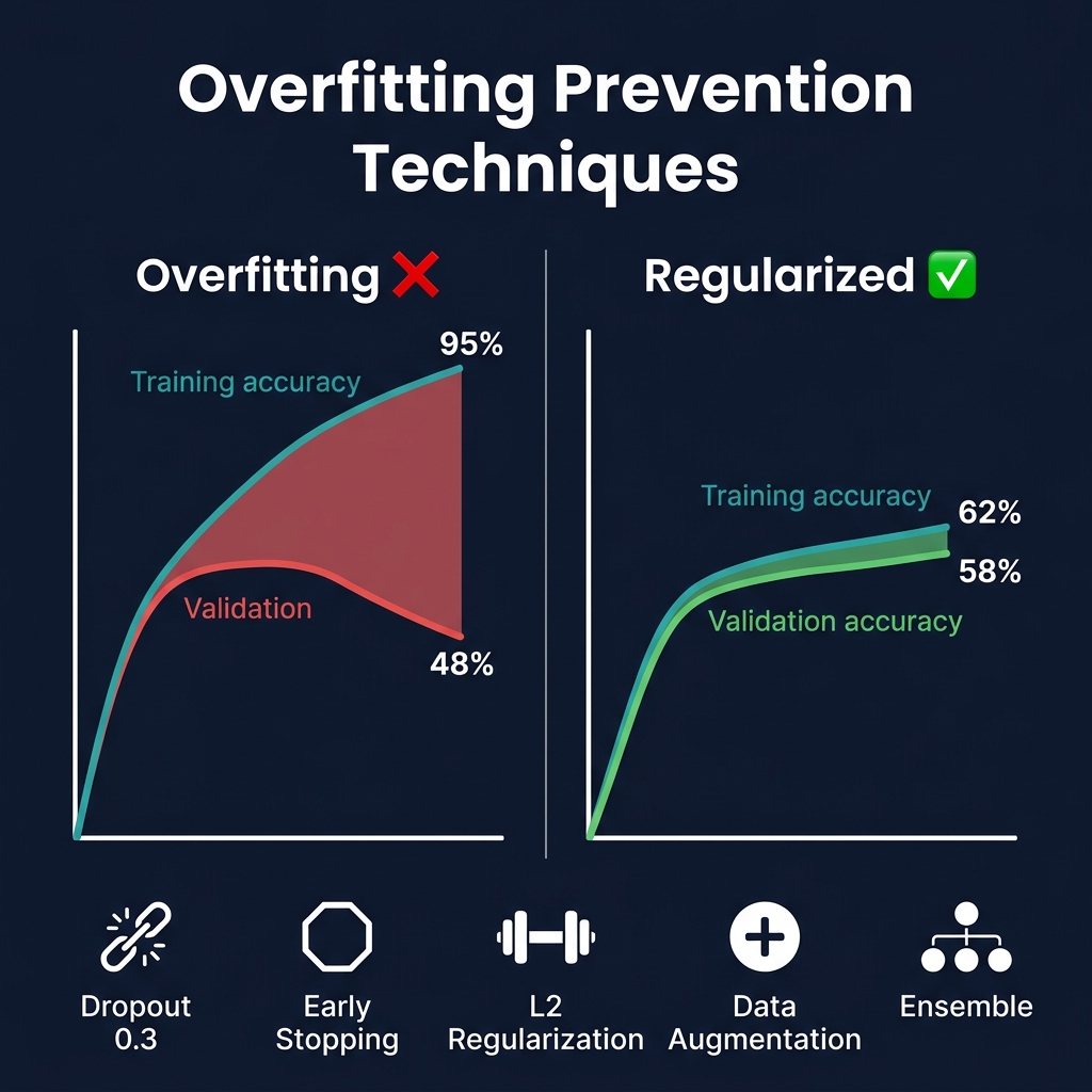
The most dangerous mistake. Your model achieves 70% accuracy in backtest and 48% live. What happened?

Overfitting indicators:

• Training accuracy >> Validation accuracy (by more than 5%)
• Performance degrades sharply on data after the training period
• Model makes extreme predictions (99% confidence) frequently
• Adding more training data doesn't improve performance

Prevention protocol:

Technique	What It Does
Dropout (0.2-0.4)	Randomly disables neurons during training, forcing redundancy
Early stopping	Stops training when validation loss increases for 5+ epochs
L2 regularization	Penalizes large weights, keeping model simple
Data augmentation	Adds noise to training data, improving generalization
Ensemble averaging	Averages predictions from 3-5 independently trained models
Walk-forward validation	Tests on future data the model has never seen

Sin 4: Predicting Price Instead of Edge

Don't try to predict the exact price. Predict something actionable:

Bad Target	Good Target	Why
"BTC will be $68,500"	"BTC has 62% probability of being above current price in 4h"	Probability is more honest and useful for sizing
"ETH price in 24 hours"	"ETH volatility will exceed 2× average in the next 6h"	Volatility prediction is more reliable and useful for stop placement
"Exact bottom"	"Current drawdown is 80th percentile — high probability of mean reversion within 48h"	Regime prediction beats point prediction

Sin 5: No Walk-Forward Validation

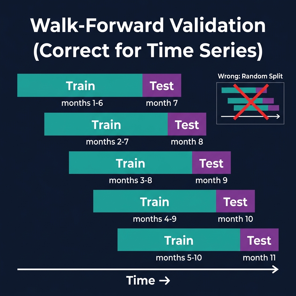
Standard train/test splits are WRONG for time series. If you randomly split your data, future data leaks into the training set.

Correct approach: Walk-Forward Validation

Period 1: Train on months 1-6,  Validate on month 7
Period 2: Train on months 2-7,  Validate on month 8  
Period 3: Train on months 3-8,  Validate on month 9
Period 4: Train on months 4-9,  Validate on month 10
...

Final metric = Average performance across ALL validation periods

This simulates real-world deployment where you only have past data for training and must predict the future.

Sin 6: Ignoring Transaction Costs

A model that generates 50 trades per day with 51% accuracy will lose money after fees. Always include realistic costs in your evaluation:

Net profit = Gross profit - (Number of trades × Average cost per trade)

Where average cost includes:
  - Exchange fee: 0.04-0.10% per trade
  - Slippage: 0.02-0.20% per trade (depends on liquidity)
  - Spread: 0.01-0.05% per trade
  
Total cost per round-trip: 0.14-0.70%

A model needs at least 0.14-0.70% edge per trade just to break even. This eliminates most "high-frequency" neural network strategies unless you're a market maker.

Sin 7: Deploying Without Monitoring

Neural networks degrade silently. Performance drops gradually as market conditions shift away from training data — you won't notice until you've lost significant capital.

Monitoring checklist:

Metric	Check Frequency	Alert Threshold
Live accuracy vs. backtest	Daily	Difference > 5% for 3+ days
Prediction confidence	Every prediction	Average confidence < 55%
Feature distribution shift	Daily	KL divergence > 0.1
Drawdown attribution	Weekly	> 50% of drawdown from AI signals
Model retraining trigger	Automatic	Rolling accuracy below 50% for 5 days

Practical Implementation Guide

Step 1: Data Pipeline

Before building any model, you need a reliable data pipeline:

Data Sources:
  ├── Price data: Binance API (1m, 5m, 1h, 4h, 1d candles)
  ├── On-chain: Glassnode/CryptoQuant API
  ├── Sentiment: LunarCrush / custom NLP on Crypto Twitter  
  ├── Macro: FRED API (DXY, yields, VIX)
  └── Calendar: Manual curation (halving, upgrades, FOMC)

Processing:
  ├── Cleaning: Handle missing data, outliers, exchange downtime
  ├── Feature engineering: Technical indicators, rolling statistics
  ├── Normalization: Z-score with 30-day rolling window
  └── Storage: Parquet files with versioning

Step 2: Choose Your Architecture

If your goal is…	Use this architecture	Why
Short-term direction (< 4h)	LSTM or GRU	Fast training, good for short sequences
Chart pattern detection	2D CNN (ResNet backbone)	Spatial pattern recognition
Multi-horizon forecasting	Temporal Fusion Transformer	Handles mixed inputs, quantile output
Production system	Ensemble of specialists	Robustness through diversity
First prototype	Simple LSTM	Fast to build, easy to debug

Step 3: Training Protocol

1. Split data: 70% train / 15% validation / 15% test (chronological!)
2. Feature selection: Start with all features, prune using importance scores
3. Hyperparameter search: Learning rate, layers, dropout, batch size
4. Training:
   - Optimizer: AdamW with cosine annealing learning rate
   - Early stopping: patience = 10 epochs
   - Batch size: 64-256 (larger = more stable training)
5. Validation:
   - Walk-forward across 6+ periods
   - Include transaction costs in all metrics
6. Ensemble:
   - Train 5 models with different random seeds
   - Average predictions (reduces variance by ~40%)

Step 4: Signal Generation

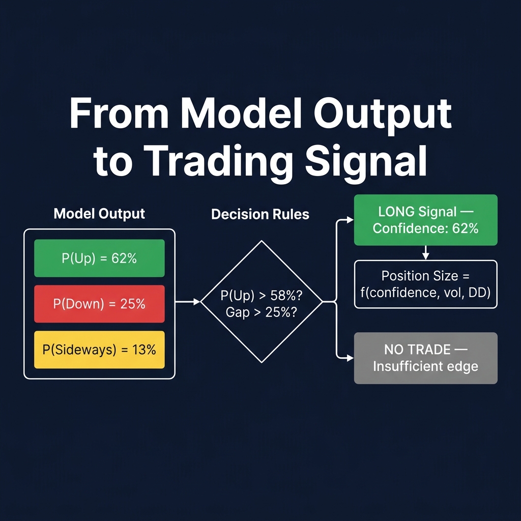
Don't trade raw model output. Convert predictions into actionable signals:

Model output: P(up) = 0.62, P(down) = 0.25, P(sideways) = 0.13

Signal rules:
  IF P(up) > 0.58 AND P(up) - P(down) > 0.25:
    Signal = LONG, Confidence = P(up)
  
  IF P(down) > 0.58 AND P(down) - P(up) > 0.25:
    Signal = SHORT, Confidence = P(down)
  
  ELSE:
    Signal = NO TRADE (insufficient edge)

Position size = f(Confidence, Volatility, Current drawdown)
  → Uses Kelly Criterion with AI risk adjustments
  → See: AI Risk Management guide

Step 5: Deployment & Monitoring

Deployment checklist:
  □ Paper trade for minimum 2 weeks
  □ Compare paper results to backtest expectations  
  □ Start with 10% of intended capital
  □ Scale up over 4-6 weeks if performance matches
  □ Set automatic model retraining schedule (weekly)
  □ Configure drift detection alerts
  □ Define kill switch: stop trading if rolling 5-day Sharpe < -1.0

3 Real Scenarios: How Neural Network Signals Played Out

Scenario 1: ETH Direction Prediction — LSTM Signal, April 12, 2026

CoinXSight's LSTM model on ETH/USDT 4H data generated a short-term bearish signal:

• Model output: P(down) = 64%, P(up) = 22%, P(sideways) = 14%
• Trigger: ETH at $2,650, RSI at 74 (overbought), funding rates at +0.08% (over-leveraged longs)
• ASI Score: 38/100 — weak multi-factor alignment

Action taken under decision rules: P(down) > 58% AND confidence spread > 25% → SHORT signal confirmed. Entry at $2,645, stop at $2,710 (above recent high), TP at $2,560.

Result: ETH dropped to $2,548 over 36 hours. TP hit for +3.7% gain. R:R achieved = 1:1.5.

Lesson: The LSTM's short-term direction call was accurate because multiple indicators confirmed. Without the Confluence Score alignment, this would have been a skip.

Scenario 2: BTC Range Prediction — TFT Quantile Output, May 1, 2026

The Temporal Fusion Transformer generated a 4-hour BTC range prediction:

• 10th percentile: $104,200 (worst case)
• 50th percentile: $105,800 (most likely)
• 90th percentile: $107,100 (best case)
• Range width: $2,900 (≈ 2.7%) — moderate confidence

Action: Range was narrow enough to justify a mean-reversion trade. BTC was at $105,100 (below the 50th percentile). Set buy limit at $104,500 with stop at $103,900 and TP at $106,500.

Result: BTC dipped to $104,350 (just missed the limit), then rallied to $106,800. A wider entry zone ($104,700) would have captured this move.

Lesson: TFT quantile output is best used for range trading and stop placement — not for directional bets. Size positions inverse to the range width: narrow range = larger position, wide range = smaller position.

Scenario 3: LINK Ensemble Regime Detection — April 28, 2026

CoinXSight's ensemble detected a regime change on LINK:

• Previous 30 days: Ranging regime (sideways between $14.20-$16.80)
• Regime classifier shifted to: Trending regime on April 28
• Catalyst: Ensemble detected increasing momentum, whale accumulation of 2.1M LINK to cold storage, and funding rates normalizing from negative

Action: Switch from range-trading strategy to trend-following. Enter long at $15.90 (breakout of range midpoint), trailing stop at 2x ATR.

Result: LINK rallied to $19.40 over 11 days (+22%). The trailing stop captured $18.80 (+18.2%).

Lesson: Regime detection is the highest-value use of neural networks. A model that tells you "the market changed" is more useful than a model that predicts a specific price. Always check CoinXSight's AI Analysis module for regime flags.

---

Your Daily Workflow: Using Neural Network Signals

Step 1: Check Regime (2 minutes)

Open CoinXSight Dashboard. The AI Analysis section shows the current market regime for BTC and your top watchlist tokens. Regime determines your strategy selection:

Regime	Strategy	Stop Type	Position Size
Trending	Ride momentum, trail stops	ATR trailing (2x)	Standard (1%)
Ranging	Mean-reversion, fade extremes	Fixed at range boundary	Smaller (0.5%)
Volatile/Chaotic	Sit out or reduce exposure	Wider stops (3x ATR)	Minimal (0.25%)

Step 2: Read Model Signals (3 minutes)

For tokens in your watchlist:

• Check ASI Score — combines all neural network outputs into one number
• Check individual dimension scores — look for divergences (Trend high but Momentum low = warning)
• Check confidence level — only act on signals where P(direction) > 58%

Step 3: Apply Decision Rules

Signal Condition	Action
P(direction) > 62% AND ASI > 70 AND Confluence ≥ 7/10	Full trade — 1.5% risk
P(direction) > 58% AND ASI 50-70	Standard trade — 1% risk
P(direction) 50-58% OR ASI < 50	Watch only — set alerts
P(direction) < 50%	No trade — model sees no edge
Regime = Chaotic	Reduce all positions by 50% regardless of signals

---

Neural networks are powerful tools, not magic oracles. They don't predict the future — they detect patterns that give you a statistical edge. A 55% accurate model with disciplined risk management will outperform a 65% accurate model with reckless sizing.

Check your tokens' AI scores now → CoinXSight AI Analysis